
NASA Selects Participants to Track Artemis II Mission
NASA has selected 34 global volunteers to track the Orion spacecraft during the crewed Artemis II mission’s journey around the Moon.
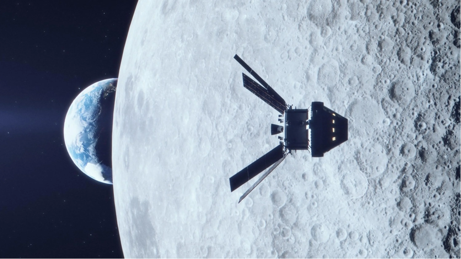
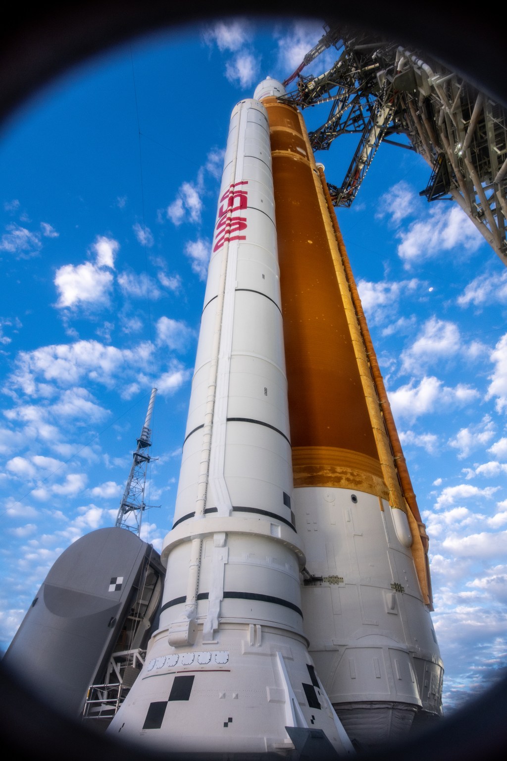
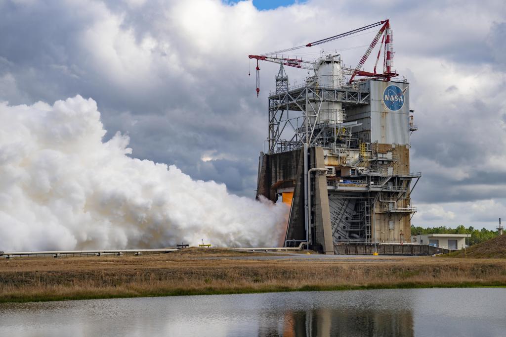
The Artemis II test flight will launch NASA’s Space Launch System (SLS) rocket, carrying the Orion spacecraft and a crew of four astronauts, on a mission into deep space. The agency’s second mission in the Artemis campaign is a key step in NASA’s path toward establishing a long-term presence at the Moon and confirming the systems needed to support future lunar surface exploration and paving the way for the first crewed mission to Mars.
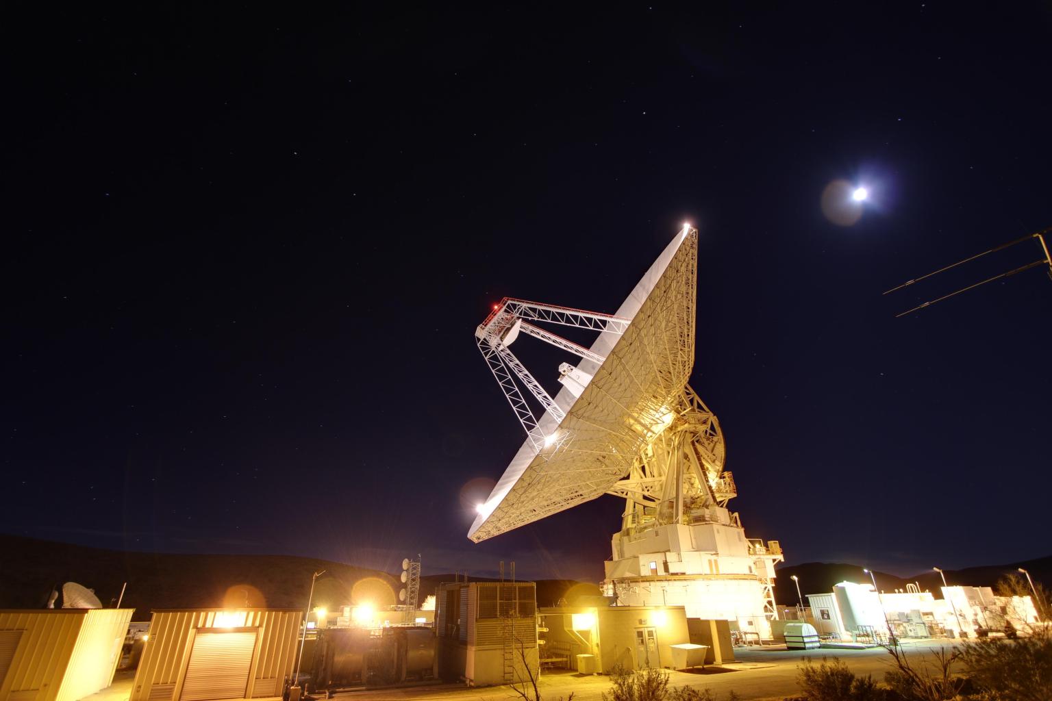
While NASA’s Near Space Network and Deep Space Network, coordinated by the agency’s SCaN (Space Communication and Navigation) program , will provide primary communications and tracking services to support Orion’s launch, journey around the Moon, and return to Earth, participants selected from a request for proposals published in August 2025, comprised of established commercial service providers, members of academia, and individual amateur radio enthusiasts will use their respective equipment to passively track radio waves transmitted by Orion during its approximately 10-day journey.
“The Artemis II tracking opportunity is a real step toward SCaN’s commercial-first vision. By inviting external organizations to demonstrate their capabilities during a human spaceflight mission, we’re strengthening the marketplace we’ll rely on as we explore farther into the solar system,” said Kevin Coggins, deputy associate administrator for SCaN at NASA Headquarters in Washington. “This isn’t about tracking one mission, but about building a resilient, public-private ecosystem that will support the Golden Age of innovation and exploration.”
This isn’t about tracking one mission, but about building a resilient, public-private ecosystem that will support the Golden Age of innovation and exploration.”

KEvin Coggins
NASA Deputy Associate Administrator for SCaN
These volunteers will submit their data to NASA for analysis, helping the agency better assess the broader aerospace community’s tracking capabilities and identify ways to augment future Moon and Mars mission support. There are no funds exchanged as a part of this collaborative effort.
This initiative builds on a previous effort in which 10 volunteers successfully tracked the Orion spacecraft during Artemis I in 2022. That campaign produced valuable data and lessons learned, including implementation, formatting, and data quality variations for Consultative Committee for Space Data Systems, which develops communications and data standards for spaceflight. To address these findings, SCaN now requires that all tracking data submitted for Artemis II comply with its data system standards.
Compared to the previous opportunity, public interest in tracking the Artemis II mission has increased. About 47 ground assets spanning 14 different countries will be used for to track the spacecraft during its journey around the Moon.
Participants List:
Government:
- Canadian Space Agency (CSA), Canada
- The German Aerospace Center (DLR), Germany
Commercial:
- Goonhilly Earth Station Ltd, United Kingdom
- GovSmart, Charlottesville, Virginia
- Integrasys + University of Seville, Spain
- Intuitive Machines, Houston
- Kongsberg Satellite Services, Norway
- Raven Defense Corporation, Albuquerque, New Mexico
- Reca Space Agency + University of Douala, Cameroon
- Rincon Research Corporation & the University of Arizona, Tucson
- Sky Perfect JSAT, Japan
- Space Operations New Zealand Limited, New Zealand
- Telespazio, Italy
- ViaSat, Carlsbad, California
- Von Storch Engineering, Netherlands
Individual:
- Chris Swier, South Dakota
- Dan Slater, California
- Loretta A Smalls, California
- Scott Tilley, Canada
Academia:
- American University, Washington
- Awara Space Center + Fukui University of Technology, Japan
- Morehead State University, Morehead, Kentucky
- Pisgah Astronomical Research Institute, Rosman, North Carolina
- University of California Berkeley, Space Sciences Laboratory, California
- University of New Brunswick, ECE, Canada
- University of Pittsburgh, ECE, Pittsburgh
- University of Zurich – Physics Department, Switzerland
Non-Profit & Amateur Radio Organizations:
- AMSAT Argentina, Argentina
- AMSAT Deutschland, Germany
- Amateur Radio Exploration Ground Station Consortium, Springfield, Illinois
- CAMRAS, Netherlands
- Deep Space Exploration Society, Kiowa County, Colorado
- Neu Golm Ground Station, Germany
- Observation Radio Pleumur-bodou, France
Artemis II will fly around the Moon to test the systems which will carry astronauts to the lunar surface for economic benefits and scientific discovery in the Golden Age of exploration and innovation.
The networks supporting Artemis receive programmatic oversight from NASA’s SCaN Program office. In addition to providing communications services to missions, SCaN develops the technologies and capabilities that will help propel NASA to the Moon, Mars, and beyond. The Deep Space Network is managed by NASA’s Jet Propulsion Laboratory in Southern California, and the Near Space Network is managed by NASA’s Goddard Space Flight Center in Greenbelt, Maryland.
Learn more about NASA’s SCaN Program:
Details
About the Author

Katrina Lee
Katrina Lee is a writer for the Space Communications and Navigation (SCaN) Program office and covers emerging technologies, commercialization efforts, exploration activities, and more.
Discover More Topics From NASA


from NASA https://ift.tt/65BMUcZ


